Card Shuffling II – The Riffle Shuffle

In my previous post on card shuffling, I established a basic framework in which we will work. We are given a probability distribution $P$ on $S_n$ and we wish to determine when $||P_k-U||$ first begins to decay exponentially, where $P_k$ is the $k$ -fold convolution of $P.$ One key feature of card shuffling theory, as well as much of finite Markov chains in general, is that the tools available are often very particular to a small class of problems. There just aren’t very many big hammers around. Even though the theorem described in the previous post was quite general, it was non-quantitative, and so not especially useful in practice.

The standard shuffling technique is called the “riffle shuffle.” In this shuffle, the deck is cut in half, and the two halves are zippered together. We need to come up with a mathematical way of describing the riffle shuffle, and I’ll list three different methods (I’m assuming the deck has $52$ cards here, but any $n$ will do):

First Way. The first thing to think about is how we cut the deck. Mathematically speaking, we will assume the number of cards in the top half of the deck after we cut is binomially distributed. All this means is that to determine the number of cards we cut from the top, flip 52 coins and count the number of heads to figure out how many cards go in the top half. It may seem strange that there is a positive probability of having all 52 cards in the deck sitting in the “top half” but the probability is extremely small and so doesn’t matter so much. For most shufflers, the size of the two “halves” are often quite different. Anyway, suppose that our result is $k$ cards in the top half. From here, we think of having 52 boxes lined up and put the cards in them. We pick $k$ of the boxes (assuming each box is equally likely) and put the top half of the deck in those boxes, keeping them in the same order. Put the remaining $52-k$ cards in the remaining boxes, keeping them in the same order relative to each other. Stack the cards back up. Note that there are $\displaystyle{\binom{52}{k}=\frac{52!}{k!(52-k)!}}$ ways to put $k$ cards in 52 boxes, so that the probability of any box choice is $1/ \binom{52}{k}$ .

Second Way. Cut the deck into two halves just like before (according to a binomial distribution). Suppose that $k$ cards are in the left hand and $52-k$ cards in the right hand. We decide to drop a card from the the left hand with probability $k/52$ and from the right hand with probability $(52-k)/52.$ If a card from the left hand drops, then we do the same thing: drop a card from the left hand now with probability $(k-1)/51$ and from the right hand with probability $(52-k)/51.$ In other words, the probability at each step that we drop from the left hand or the right hand will be proportional to the number of cards in the left hand or right hand. Continue this process until all the cards have been dropped.

Third Way. This is the inverse shuffle. For each card in the deck, flip a coin and label the back of the card H or T depending on whether the coin landed heads or tails. Take all the cards labeled H out of the deck, maintaining them in relative order to one another and put them on top. This is another way to think of the riffle shuffle (even though it seems strange).

Each of these ways to view the riffle shuffle is actually the same in the sense that if we start at a particular order, the probability of getting the deck into any particular new ordering is the same in all three shuffles. To see that #1 and #2 are the same, observe that one flips coins in the same way. Assuming that $k$ heads come up, exactly $k$ cards end up in the left hand and $52-k$ cards in the right hand. In #1, one ends up with a sequence of 52 L’s and R’s: the first is an L if the top card after the shuffle came from the left hand and R if it came from the right. Likewise with the second entry, and so on. Each of these orderings is equally likely. In #2, one ends up with a sequence of L’s and R’s depending on the order in which the cards dropped. The probability of any particular ordering is always $\displaystyle{\frac{k!(52-k)!}{52!}=\frac{1}{\binom{52}{k}}}$ , which is the same as the probability we found in #1. To see that #1 and #3 are the same, notice that we end up with a sequence of L’s and R’s and H’s and T’s. For the moment, assume that L=H and R=T. Then we end up with the same possible subset of sequences. The probability of each sequence is the same since in each case each choice has the same probability and there are the same number of sequences possible.

This model of the riffle shuffle is rather good for amateur shufflers. Professionals (casino dealers, magicians, and so forth) are not modeled quite as well by this technique since they tend to have less variation in the size of each half of the deck and also tend to be able to have one card drop from one hand and then one card drop from the other. But for the casual card player, this is just about enough.

It is worth noting at this point, that if one were to view shuffles as a Markov chain, the matrix produced by the riffle shuffle is, first, gigantic ( $n! \times n!$ ), and, second, hard to write down regardless. So, it seems like estimating the decay from the point-of-view of analyzing the behavior of the second-largest eigenvalue would be difficult in this case. Let’s try a different means of attacking the problem.

To derive the an upper bound on the number of times one has to shuffle to start decaying exponentially to the uniform distribution we will make use of a technical lemma. But first, one needs a couple of definitions, the first of which being one that probably any mathematician should know. I’m writing the definition with respect to this problem, but the basic idea is the same, for the most part, even in more general situations.

Definition. Stopping Time
A stopping time $T$ is an integer-valued function defined on the sequence space of shuffles. One gives the stopping time a sequence of shuffles as input and the stopping time looks for the first shuffle in the sequence for which a particular condition is satisfied. If the $m^{\textrm{th}}$ shuffle is where this occurs, then the stopping time outputs $m$ . The key technical property of $T$ is that it only requires finite information. In particular, if for a sequence $\bar{g}$ , $T(\bar{g})=m$ , then $T(\bar{h})=m$ for any sequence $\bar{h}$ which agrees with $\bar{g}$ in the first $m$ entries. As an example, we might say, “Stop when the deck has an ace on top.” Then we keep shuffling the deck, keep track of how many times we’ve shuffled, and then write down how many times we had to wait until an ace was on top.

Definition. Strong Uniform Time
Suppose we have a stopping time $T$ . Let $X_k$ denote the order of our deck after $k$ shuffles. $T$ is a strong uniform time if the probability that $T=k$ and $X_k=s$ , simultaneously, is constant in $s$ . In other words, the outcomes of $k$ shuffles under the requirement that $T=k$ all are equally likely. It can be slightly confusing to think about what the probability that $T=k$ means. One has to define a probability on the sequences of shuffles (state space). I won’t do that here, but there are plenty of references out there that can if you’re really curious.

Here is a lemma from Persi Diaconis’s book, Group Representations in Probability and Statistics, 1988:

Lemma. Let $P$ be any probability distribution defined a finite group, $G.$ Let $T$ be a strong uniform time for $P$ . Then for all $k\ge 0$ ,

$\displaystyle{||P_k -U||\le Pr(T>k)}$ .

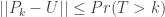The proof of the lemma is clever but not very hard — and not especially enlightening either (see page 70 of Diaconis’s book if interested). What it does give us is a way to use a strong stopping time to produce an upper bound estimate on the number of shuffles required. So, we have two goals now: construct a strong uniform time for the riffle shuffle and then compute the probability that it is bigger than $k$ .

We construct the uniform stopping time as follows. List the $n$ cards of the deck as the rows of a matrix. We perform repeated inverse shuffles. At each shuffle, add an additional column to the matrix. Put an H (or T) in the row for each card if in that shuffle, that card was associated with a heads (or tails). The rows of the columns produce a way to order the cards. For instance — looking at the first two columns of our matrix — cards which have HH are above cards which are TH. TH cards are above HT cards, and TT cards are all on the bottom. For the first three columns, the ordering would be HHH, THH, HTH, TTH, HHT, THT, HTT, TTT.

For a sequence of shuffles, we construct a (very large) matrix $A$ . Let $T$ be defined on sequences of shuffles so that $T=k$ when $k$ is the minimum number of columns necessary to make the rows of $A$ distinct (that is, no two rows are exactly the same). For 52 cards, $T\ge 6$ . $T$ is a stopping time because if $T=10$ , we are able to determine this based on just the first 10 shuffles (we just need the first 10 columns of $A$ , after all).

$T$ is a strong uniform time because, assuming that $T=k$ , one could easily interchange any rows in the matrix $A$ to produce an equally valid sequence of (inverse) riffle shuffles which still has $T=k$ . Since the sequence in each row determines the position of each card in the deck, this gives us a way to produce any ordering of the deck, and thus there are $n!$ ways of reordering the rows. But the sequence of shuffles which have the same rows as our matrix $A$ are all equally likely, and so the probability of getting a particular outcome $X_k$ , assuming $T=k$ , has probability $1/n!$ . Hence $T$ is a strong uniform time.

The situation we are in with $Pr(T>k)$ is similar to the Birthday Problem. Here we think of the cards as people and think of their associated rows as their birthdays. $Pr(T>k)$ is the probability that at least two cards have the same rows of length $k$ : there are $2^k$ rows of length $k$ (since there are 2 possibilities for each entry, H or T), and thus $2^k$ birthdays. There are $n$ cards. Hence

$\displaystyle{Pr(T>k)= 1-\prod_{i=1}^{n-1}(1-\frac{i}{2^k})}.$

By choosing $k=2\log_2 n$ , and applying some simple manipulations, one can see that for large $n$ ,

$\displaystyle{1-\prod_{i=1}^{n-1}(1-\frac{i}{2^k})\approx 1-e^{-1/2}\le 1/2.}$

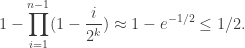
So, we need at most $2\log_2 n$ shuffles, provided $n$ is large enough (note that $n=52$ is “large enough”). In 1983, David Aldous made a much more careful analysis to determine that $\frac{3}{2}\log_2 n$ is actually sufficient for large $n$ . For $n=52$ , this number is approximately 8.5, so somewhere around 8 shuffles should suffice.

This entry was posted on April 21, 2009 at 12:08 am and is filed under Basic Grad Student, Guests. You can follow any responses to this entry through the RSS 2.0 feed. You can leave a response, or trackback from your own site.

3 Responses to “Card Shuffling II – The Riffle Shuffle”

How many dovetail shuffles suffice? « Rod Carvalho's web notebook Says:
December 18, 2009 at 2:22 am | Reply
[…] Card Shuffling II – The Riffle Shuffle […]
Камеры Видеонаблюдения Says:
September 15, 2010 at 7:36 am | Reply
thank you, very good description
prof dr mircea orasanu Says:
May 31, 2019 at 11:33 am | Reply
these are very important observed prof dr mircea orasanu and prof drd horia orasanu

The Everything Seminar